Vibrational strong coupling with liquid water: Unix socket

Here, we introduce how to use MaxwellLink to run cavity molecular dynamics (CavMD) simulations of liquid water under vibrational strong coupling.

1. Setting up the socket communication layer

Using the TCP socket requires to set the hostname and port number. In local machines, we can use the helper function get_available_host_port() from MaxwellLink to obtain these two pieces of information. Then, we initialize a SocketHub instance to provide the socket communication in MaxwellLink.

import numpy as np
import maxwelllink as mxl

address = "socket_cavmd"
hub = mxl.SocketHub(unixsocket=address, timeout=10.0, latency=1e-5)

2. Bind Molecule and EM solver to the SocketHub

Then, we create a Molecule instance to define the information of this molecule in the EM simulation environment. We also need to setup the EM solver (MEEP) as a classical single mode cavity using mxl.SingleModeSimulation.

# the rescaling 0.73 is to account for the difference between the TIP4P water model verus that from a straightforward
# sum_i Q_i * r_i calculation, where the oxygen atom is used for the position instead of using the M charge site.
# In other words, the dipole and dmudt calculation from MD driver needs to be rescaled by 0.73 to match the real TIP4P
# water model values (used in i-pi CavMD).
molecule = mxl.Molecule(
    hub=hub,
    rescaling_factor=0.73,
)

au_to_cminverse = 219474.63

frequency_au = 3550 / au_to_cminverse
coupling_strength = 4e-4
print(f"Coupling strength: {coupling_strength:.3e} au")
damping_au = 0e-4
fs_to_au = 41.3413745758
dt_fs = 0.5
dt_au = dt_fs * fs_to_au

sim = mxl.SingleModeSimulation(
    hub=hub,
    molecules=[molecule],
    frequency_au=frequency_au,
    coupling_strength=coupling_strength,
    damping_au=damping_au,
    coupling_axis="z",
    drive=0.0,
    dt_au=dt_au,
    record_history=True,
    include_dse=True,
)

[Init Molecule] Under socket mode, registered molecule with ID 0
Coupling strength: 4.000e-04 au

3. Python way to lunch LAMMPS on a separate terminal

Generally, using the Socket Interface requires to launch the EM simulation in one terminal and then start the molecular driver simulation in a separate terminal. To avoid openning a second terminal, below we introduce a python helper function launch_lmp(...), which will launch LAMMPS (the lmp_mxl binary file) from Python (so we can stay within this notebook to finish this tutorial).

The LAMMPS code performs a 10-ps NVE liquid water simulation. The fix mxl command in the LAMMPS input file communicates between LAMMPS and MaxwellLink.

In a 2021 MacBook Pro M1, this simulation takes approximately 1.5 minutes.

import shlex
import subprocess
import time


def launch_lmp(address: str, sleep_time: float = 0.5):
    cmd = (
        f"./lmp_input/launch_lmp_xml.sh {address} "
    )
    print('Launching LMP via subprocess...')
    print('If you prefer to run it manually, execute:')
    print('  ' + cmd)
    argv = shlex.split(cmd)
    proc = subprocess.Popen(argv)
    time.sleep(sleep_time)
    return proc

launch_lmp(address)

sim.run(steps=int(10000/dt_fs))

Launching LMP via subprocess...
If you prefer to run it manually, execute:
  ./lmp_input/launch_lmp_xml.sh socket_cavmd
Preparing LAMMPS input files with port socket_cavmd...
LAMMPS (29 Aug 2024 - Update 1)
Reading data file ...
  orthogonal box = (0 0 0) to (35.233 35.233 35.233)
  1 by 1 by 1 MPI processor grid
  reading atoms ...
  648 atoms
  scanning bonds ...
  2 = max bonds/atom
  scanning angles ...
  1 = max angles/atom
  orthogonal box = (0 0 0) to (35.233 35.233 35.233)
  1 by 1 by 1 MPI processor grid
  reading bonds ...
  432 bonds
  reading angles ...
  216 angles
Finding 1-2 1-3 1-4 neighbors ...
  special bond factors lj:    0        0        0
  special bond factors coul:  0        0        0
     2 = max # of 1-2 neighbors
     1 = max # of 1-3 neighbors
     1 = max # of 1-4 neighbors
     2 = max # of special neighbors
  special bonds CPU = 0.000 seconds
  read_data CPU = 0.004 seconds
[MaxwellLink] Will reset initial permanent dipole to zero.

CITE-CITE-CITE-CITE-CITE-CITE-CITE-CITE-CITE-CITE-CITE-CITE-CITE

Your simulation uses code contributions which should be cited:
- Type Label Framework: https://doi.org/10.1021/acs.jpcb.3c08419
The log file lists these citations in BibTeX format.

CITE-CITE-CITE-CITE-CITE-CITE-CITE-CITE-CITE-CITE-CITE-CITE-CITE

PPPM initialization ...
  extracting TIP4P info from pair style
  using 12-bit tables for long-range coulomb (src/kspace.cpp:342)
  G vector (1/distance) = 0.16615131
  grid = 15 15 15
  stencil order = 5
  estimated absolute RMS force accuracy = 1.3905979e-05
  estimated relative force accuracy = 4.9659152e-05
  using double precision KISS FFT
  3d grid and FFT values/proc = 10648 3375
WARNING: Communication cutoff 0 is shorter than a bond length based estimate of 4.67. This may lead to errors. (src/comm.cpp:730)
WARNING: Increasing communication cutoff to 21.065072 for TIP4P pair style (src/KSPACE/pair_lj_cut_tip4p_long.cpp:497)
Generated 0 of 1 mixed pair_coeff terms from geometric mixing rule
Neighbor list info ...
  update: every = 1 steps, delay = 0 steps, check = yes
  max neighbors/atom: 2000, page size: 100000
  master list distance cutoff = 19.563145
  ghost atom cutoff = 21.065072
  binsize = 9.7815724, bins = 4 4 4
  1 neighbor lists, perpetual/occasional/extra = 1 0 0
  (1) pair lj/cut/tip4p/long, perpetual
      attributes: half, newton on
      pair build: half/bin/newton
      stencil: half/bin/3d
      bin: standard
Setting up Verlet run ...
  Unit style    : electron
  Current step  : 0
  Time step     : 0.5
Per MPI rank memory allocation (min/avg/max) = 8.721 | 8.721 | 8.721 Mbytes
   Step          Temp          E_pair         E_mol          TotEng         Press
         0   300           -4.0744255      0.58197053    -2.5704367      71675325
[SocketHub][MaxwellLink] Assigned a molecular ID: 0
[MaxwellLink] 1 atomic units time in LAMMPS native time units = 0.024188843265864
[MaxwellLink] MaxwellLink uses time step: dt_au = 20.6706872879 ->  dt_native (LAMMPS units) = 0.5000000150047
[MaxwellLink] Modified LAMMPS time step from 0.5 to 0.5000000150047 to match MaxwellLink dt!
[MaxwellLink] Make sure all coupled simulations use this time step, after the modification, LAMMPS dt = 0.5000000150047!
 CONNECTED: mol 0 <-
[SingleModeCavity] Completed 1000/20000 [5.0%] steps, time/step: 4.95e-03 seconds, remaining time: 94.03 seconds.
[SingleModeCavity] Completed 2000/20000 [10.0%] steps, time/step: 4.83e-03 seconds, remaining time: 87.96 seconds.
[SingleModeCavity] Completed 3000/20000 [15.0%] steps, time/step: 4.50e-03 seconds, remaining time: 80.91 seconds.
[SingleModeCavity] Completed 4000/20000 [20.0%] steps, time/step: 4.51e-03 seconds, remaining time: 75.15 seconds.
[SingleModeCavity] Completed 5000/20000 [25.0%] steps, time/step: 4.54e-03 seconds, remaining time: 69.97 seconds.
[SingleModeCavity] Completed 6000/20000 [30.0%] steps, time/step: 4.84e-03 seconds, remaining time: 65.72 seconds.
[SingleModeCavity] Completed 7000/20000 [35.0%] steps, time/step: 4.63e-03 seconds, remaining time: 60.91 seconds.
[SingleModeCavity] Completed 8000/20000 [40.0%] steps, time/step: 4.55e-03 seconds, remaining time: 56.02 seconds.
[SingleModeCavity] Completed 9000/20000 [45.0%] steps, time/step: 4.70e-03 seconds, remaining time: 51.38 seconds.
[SingleModeCavity] Completed 10000/20000 [50.0%] steps, time/step: 4.63e-03 seconds, remaining time: 46.67 seconds.
[SingleModeCavity] Completed 11000/20000 [55.0%] steps, time/step: 4.45e-03 seconds, remaining time: 41.82 seconds.
[SingleModeCavity] Completed 12000/20000 [60.0%] steps, time/step: 4.50e-03 seconds, remaining time: 37.08 seconds.
[SingleModeCavity] Completed 13000/20000 [65.0%] steps, time/step: 4.54e-03 seconds, remaining time: 32.39 seconds.
[SingleModeCavity] Completed 14000/20000 [70.0%] steps, time/step: 4.71e-03 seconds, remaining time: 27.80 seconds.
[SingleModeCavity] Completed 15000/20000 [75.0%] steps, time/step: 4.76e-03 seconds, remaining time: 23.20 seconds.
[SingleModeCavity] Completed 16000/20000 [80.0%] steps, time/step: 4.82e-03 seconds, remaining time: 18.61 seconds.
[SingleModeCavity] Completed 17000/20000 [85.0%] steps, time/step: 4.64e-03 seconds, remaining time: 13.95 seconds.
[SingleModeCavity] Completed 18000/20000 [90.0%] steps, time/step: 4.75e-03 seconds, remaining time: 9.31 seconds.
[SingleModeCavity] Completed 19000/20000 [95.0%] steps, time/step: 4.61e-03 seconds, remaining time: 4.65 seconds.
[SingleModeCavity] Completed 20000/20000 [100.0%] steps, time/step: 4.71e-03 seconds, remaining time: 0.00 seconds.
[SocketHub] DISCONNECTED: mol 0 from
[MaxwellLink] Server requested stop/exit, exiting gracefully...
[SocketHub] Unlinked unix socket path /tmp/socketmxl_socket_cavmd

4. Retrieve molecular simulation data

After the simulation, we can retrieve molecular simulation data from molecule.additional_data_history, a Python list which stores the molecular information sent from the driver code at each step of the simulation.

for data in molecule.additional_data_history[0:5]:
    print(data)

{'time_au': 20.670687908214944, 'mux_au': -0.123007369475225, 'muy_au': 0.414604211280153, 'muz_au': -0.133248553303204, 'mux_m_au': -0.123007369475225, 'muy_m_au': 0.414604211280153, 'muz_m_au': -0.133248553303204, 'energy_au': -2.627474698462433, 'temp_K': 279.0533752828051, 'pe_au': -3.486441311034758, 'ke_au': 0.858966612572326}
{'time_au': 41.34137581642989, 'mux_au': -0.201399274240348, 'muy_au': 0.631882469775508, 'muz_au': -0.20536667495551, 'mux_m_au': -0.201399274240348, 'muy_m_au': 0.631882469775508, 'muz_m_au': -0.20536667495551, 'energy_au': -2.627623458160897, 'temp_K': 279.70744016291457, 'pe_au': -3.488603376947136, 'ke_au': 0.860979918786238}
{'time_au': 62.01206372464483, 'mux_au': -0.282723361978718, 'muy_au': 0.792759099858962, 'muz_au': -0.260936561671233, 'mux_m_au': -0.282723361978718, 'muy_m_au': 0.792759099858962, 'muz_m_au': -0.260936561671233, 'energy_au': -2.62845421472813, 'temp_K': 282.51250869263663, 'pe_au': -3.498068539783659, 'ke_au': 0.869614325055529}
{'time_au': 82.68275163285978, 'mux_au': -0.373779826045237, 'muy_au': 0.897451655095484, 'muz_au': -0.301234691244421, 'mux_m_au': -0.373779826045237, 'muy_m_au': 0.897451655095484, 'muz_m_au': -0.301234691244421, 'energy_au': -2.629616492246351, 'temp_K': 286.2048465594923, 'pe_au': -3.510596366802047, 'ke_au': 0.880979874555696}
{'time_au': 103.35343954107474, 'mux_au': -0.481356436920109, 'muy_au': 0.951785076875844, 'muz_au': -0.331109240937163, 'mux_m_au': -0.481356436920109, 'muy_m_au': 0.951785076875844, 'muz_m_au': -0.331109240937163, 'energy_au': -2.630450708796214, 'temp_K': 289.1237614974894, 'pe_au': -3.520415425316775, 'ke_au': 0.889964716520561}

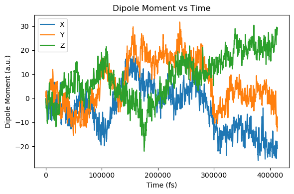
5. Plot IR spectrum

from maxwelllink.tools import ir_spectrum
import matplotlib.pyplot as plt

mux = np.array([ad["mux_m_au"] for ad in molecule.additional_data_history])[1:-1]
muy = np.array([ad["muy_m_au"] for ad in molecule.additional_data_history])[1:-1]
muz = np.array([ad["muz_m_au"] for ad in molecule.additional_data_history])[1:-1]
t = np.array([ad["time_au"] for ad in molecule.additional_data_history])[1:-1]

plt.figure(figsize=(6, 4))
plt.plot(t, mux, label="X")
plt.plot(t, muy, label="Y")
plt.plot(t, muz, label="Z")
plt.xlabel("Time (fs)")
plt.ylabel("Dipole Moment (a.u.)")
plt.title("Dipole Moment vs Time")
plt.legend()
plt.tight_layout()
plt.show()

freq, sp_x = ir_spectrum(mux, dt_fs, field_description="square")
freq, sp_y = ir_spectrum(muy, dt_fs, field_description="square")
freq, sp_z = ir_spectrum(muz, dt_fs, field_description="square")

plt.figure(figsize=(6, 4))
plt.plot(freq, sp_x, label="X")
plt.plot(freq, sp_y, label="Y")
plt.plot(freq, sp_z, label="Z")
plt.xlim(0, 5500)
plt.xlabel("Frequency (cm$^{-1}$)")
plt.ylabel("Spectral Power")
plt.title("Infrared Spectrum")
plt.legend()
plt.tight_layout()

plt.show()

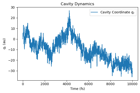
# plot cavity dynamics
au_to_fs = 41.3413745758
t = np.array(sim.time_history) / au_to_fs
# qc[0] is the z-direction cavity coordinate
qc = np.array([qc[-1] for qc in sim.qc_history])

freq, sp_qc = ir_spectrum(qc, dt_fs, field_description="square")


plt.figure(figsize=(6, 4))
plt.plot(t, qc, label="Cavity Coordinate $q_c$")
plt.xlabel("Time (fs)")
plt.ylabel("$q_c$ (au)")
plt.title("Cavity Dynamics")
plt.legend()
plt.tight_layout()
plt.show()


plt.figure(figsize=(6, 4))
plt.plot(freq, sp_qc / np.max(sp_qc), label="$q_c$")
plt.xlim(0, 8000)
plt.xlabel("Frequency (cm$^{-1}$)")
plt.ylabel("Spectrum (arb. units)")
plt.title("Photonic Spectrum")
plt.legend()
plt.tight_layout()
plt.show()

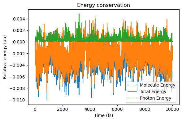
6. Energy conservation analysis

energy_molecule = np.array([ad["energy_au"] for ad in molecule.additional_data_history])
energy_tot = np.array(sim.energy_history)
energy_photon = energy_tot - energy_molecule

plt.figure(figsize=(6, 4))
plt.plot(t, energy_molecule - energy_molecule[0], label="Molecule Energy")
plt.plot(t, energy_tot - energy_tot[0], label="Total Energy")
plt.plot(t, energy_photon - energy_photon[0], label="Photon Energy")
plt.xlabel("Time (fs)")
plt.ylabel("Relative energy (au)")
plt.title("Energy conservation")
plt.legend()
plt.tight_layout()
plt.show()