Vibrational strong coupling of liquid water in a Bragg resonator: Unix socket
Authors: Xinwei Ji, Tao E. Li
Here, we introduce how to use MaxwellLink to run classical molecular dynamics (LAMMPS) simulations of liquid water under vibrational strong coupling by connecting MEEP FDTD with LAMMPS.
1. Run with realistic Bragg resonator
Let’s try to setup our simulation for an abstract Molecule confined at the center of a Bragg resonator in 1D.
This Bragg resonator is composed of a pair of parallel mirrors spaced by \(\lambda/2\), each of which consists of five periodic dielectric layers. The spacing between the neighboring dielectric layer is \(\lambda/4\). With the refrative index of each dielectric layer as \(n=2\), each dielectric layer possesses a thickness of \(\lambda/8\). This Bragg resonator supports a resonant cavity mode at wavelength \(\lambda\).
We also artifically enhance the current density of this abstract Molecule by a factor of rescaling_factor=1e5, so that strong coupling can form for a small ensemble of molecules coupled to the optical cavity. This abstract Molecule is connected to the MEEP FDTD solver via the Unix socket in local machines.
[1]:
import numpy as np
import maxwelllink as mxl
import meep as mp

address = "socket_cavmd"
hub = mxl.SocketHub(unixsocket=address, timeout=10.0, latency=1e-5)

resolution = 20
time_units_fs = 20
rescaling = 0.47

# geometry 1: 1d bragg resonator
pml_thickness = 2.0 * rescaling
t1 = 0.125 * rescaling
t2 = 0.25 * rescaling
n1 = 2.0
n2 = 1.0

nlayer = 5
layer_indexes = np.array([n2, n1] * nlayer + [1.0] + [n1, n2] * nlayer)
layer_thicknesses = np.array([t2, t1] * nlayer + [0.5 * rescaling] + [t1, t2] * nlayer)

layer_thicknesses[0] += pml_thickness
layer_thicknesses[-1] += pml_thickness
length = np.sum(layer_thicknesses)
layer_centers = np.cumsum(layer_thicknesses) - layer_thicknesses/2
layer_centers = layer_centers - length/2
cell_size = mp.Vector3(length, 0, 0)
pml_layers = [mp.PML(thickness=pml_thickness)]

geometry = [mp.Block(mp.Vector3(layer_thicknesses[i], mp.inf, mp.inf),
    center=mp.Vector3(layer_centers[i], 0, 0), material=mp.Medium(index=layer_indexes[i]))
    for i in range(layer_thicknesses.size)]

# geometry 2: 1d free space with metallic boundary conditions
# one can comment out the following block to check energy conservation
'''
length = 0.5 * rescaling
cell_size = mp.Vector3(length, 0, 0)
geometry = []
pml_layers = []
'''

molecule = mxl.Molecule(
    hub=hub,
    center=mp.Vector3(0, 0, 0),
    size=mp.Vector3(0.25, 0, 0),
    sigma=0.05,
    dimensions=1,
    rescaling_factor=1e5
)

sources_non_molecule = []
sources = sources_non_molecule + molecule.sources
sim = mxl.MeepSimulation(
    hub=hub,
    molecules=[molecule],
    cell_size=cell_size,
    resolution=resolution,
    time_units_fs=time_units_fs,
    sources=sources,
    geometry=geometry,
    boundary_layers=pml_layers
)
Using MPI version 4.1, 1 processes
[Init Molecule] Under socket mode, registered molecule with ID 0


 ######### MaxwellLink Units Helper #########
 MEEP uses its own units system, which is based on the speed of light in vacuum (c=1),
 the permittivity of free space (epsilon_0=1), and the permeability of free space (mu_0=1).
 To couple MEEP with molecular dynamics, we set [c] = [epsilon_0] = [mu_0] = [hbar] = 1.
 By further defining the time unit as 2.00E+01 fs, we can fix the units system of MEEP (mu).

 Given the simulation resolution = 20,
 - FDTD dt = 2.50E-02 mu (0.5/resolution) = 5.00E-01 fs
 - FDTD dx = 5.00E-02 mu (1.0/resolution) = 3.00E+02 nm
 - Time [t]: 1 mu = 2.00E+01 fs = 8.27E+02 a.u.
 - Length [x]: 1 mu = 6.00E+03 nm
 - Angular frequency [omega = 2 pi * f]: 1 mu = 2.0688E-01 eV = 1.6686E+03 cm-1 = 7.6027E-03 a.u.
 - Electric field [E]: 1 mu = 1.66E+03 V/m = 3.23E-09 a.u.
 Hope this helps!
 ############################################
2. Python way to lunch LAMMPS on a separate terminal
We then attach this abstract Molecule with liquid water (216 H2O molecules) simulated via the LAMMPS MD driver.
Generally, using the socket interface requires to launch the EM simulation in one terminal and then start the molecular driver simulation in a separate terminal. To avoid openning a second terminal, below we introduce a python helper function launch_lmp(...), which will launch LAMMPS (the lmp_mxl binary file) from Python (so we can stay within this notebook to finish this tutorial).
The LAMMPS code performs a NVE liquid water simulation. The fix mxl command in the LAMMPS input file communicates between LAMMPS and MaxwellLink.
In a 2021 MacBook Pro M1, this simulation takes approximately 1.5 minutes.
[2]:
import shlex
import subprocess
import time

def launch_lmp(address: str, sleep_time: float = 0.5):
    cmd = (
        f"./lmp_input/launch_lmp_xml.sh {address} "
    )
    print('Launching LAMMPS via subprocess...')
    print('If you prefer to run it manually, execute:')
    print('  ' + cmd)
    argv = shlex.split(cmd)
    proc = subprocess.Popen(argv)
    time.sleep(sleep_time)
    return proc

launch_lmp(address)

sim.run(steps=2e4)
Launching LAMMPS via subprocess...
If you prefer to run it manually, execute:
  ./lmp_input/launch_lmp_xml.sh socket_cavmd
Preparing LAMMPS input files with port socket_cavmd...
LAMMPS (29 Aug 2024 - Update 1)
Reading data file ...
  orthogonal box = (0 0 0) to (35.233 35.233 35.233)
  1 by 1 by 1 MPI processor grid
  reading atoms ...
  648 atoms
  scanning bonds ...
  2 = max bonds/atom
  scanning angles ...
  1 = max angles/atom
  orthogonal box = (0 0 0) to (35.233 35.233 35.233)
  1 by 1 by 1 MPI processor grid
  reading bonds ...
  432 bonds
  reading angles ...
  216 angles
Finding 1-2 1-3 1-4 neighbors ...
  special bond factors lj:    0        0        0
  special bond factors coul:  0        0        0
     2 = max # of 1-2 neighbors
     1 = max # of 1-3 neighbors
     1 = max # of 1-4 neighbors
     2 = max # of special neighbors
  special bonds CPU = 0.000 seconds
  read_data CPU = 0.004 seconds
[MaxwellLink] Will reset initial permanent dipole to zero.

CITE-CITE-CITE-CITE-CITE-CITE-CITE-CITE-CITE-CITE-CITE-CITE-CITE

Your simulation uses code contributions which should be cited:
- Type Label Framework: https://doi.org/10.1021/acs.jpcb.3c08419
The log file lists these citations in BibTeX format.

CITE-CITE-CITE-CITE-CITE-CITE-CITE-CITE-CITE-CITE-CITE-CITE-CITE

PPPM initialization ...
  extracting TIP4P info from pair style
  using 12-bit tables for long-range coulomb (src/kspace.cpp:342)
  G vector (1/distance) = 0.16615131
  grid = 15 15 15
  stencil order = 5
  estimated absolute RMS force accuracy = 1.3905979e-05
  estimated relative force accuracy = 4.9659152e-05
  using double precision KISS FFT
  3d grid and FFT values/proc = 10648 3375
WARNING: Communication cutoff 0 is shorter than a bond length based estimate of 4.67. This may lead to errors. (src/comm.cpp:730)
WARNING: Increasing communication cutoff to 21.065072 for TIP4P pair style (src/KSPACE/pair_lj_cut_tip4p_long.cpp:497)
Generated 0 of 1 mixed pair_coeff terms from geometric mixing rule
Neighbor list info ...
  update: every = 1 steps, delay = 0 steps, check = yes
  max neighbors/atom: 2000, page size: 100000
  master list distance cutoff = 19.563145
  ghost atom cutoff = 21.065072
  binsize = 9.7815724, bins = 4 4 4
  1 neighbor lists, perpetual/occasional/extra = 1 0 0
  (1) pair lj/cut/tip4p/long, perpetual
      attributes: half, newton on
      pair build: half/bin/newton
      stencil: half/bin/3d
      bin: standard
Setting up Verlet run ...
  Unit style    : electron
  Current step  : 0
  Time step     : 0.5
Per MPI rank memory allocation (min/avg/max) = 8.721 | 8.721 | 8.721 Mbytes
   Step          Temp          E_pair         E_mol          TotEng         Press
         0   300           -4.0744255      0.58197053    -2.5704367      71675325
Warning: grid volume is not an integer number of pixels; cell size will be rounded to nearest pixel.
-----------
Initializing structure...
time for choose_chunkdivision = 0.000111 s
Working in 2D dimensions.
Computational cell is 3.9 x 0.05 x 0 with resolution 20
     block, center = (-1.41,0,0)
          size (1.0575,1e+20,1e+20)
          axes (1,0,0), (0,1,0), (0,0,1)
          dielectric constant epsilon diagonal = (1,1,1)
     block, center = (-0.851875,0,0)
          size (0.05875,1e+20,1e+20)
          axes (1,0,0), (0,1,0), (0,0,1)
          dielectric constant epsilon diagonal = (4,4,4)
     block, center = (-0.76375,0,0)
          size (0.1175,1e+20,1e+20)
          axes (1,0,0), (0,1,0), (0,0,1)
          dielectric constant epsilon diagonal = (1,1,1)
     block, center = (-0.675625,0,0)
          size (0.05875,1e+20,1e+20)
          axes (1,0,0), (0,1,0), (0,0,1)
          dielectric constant epsilon diagonal = (4,4,4)
     block, center = (-0.5875,0,0)
          size (0.1175,1e+20,1e+20)
          axes (1,0,0), (0,1,0), (0,0,1)
          dielectric constant epsilon diagonal = (1,1,1)
     block, center = (-0.499375,0,0)
          size (0.05875,1e+20,1e+20)
          axes (1,0,0), (0,1,0), (0,0,1)
          dielectric constant epsilon diagonal = (4,4,4)
     block, center = (-0.41125,0,0)
          size (0.1175,1e+20,1e+20)
          axes (1,0,0), (0,1,0), (0,0,1)
          dielectric constant epsilon diagonal = (1,1,1)
     block, center = (-0.323125,0,0)
          size (0.05875,1e+20,1e+20)
          axes (1,0,0), (0,1,0), (0,0,1)
          dielectric constant epsilon diagonal = (4,4,4)
     block, center = (-0.235,0,0)
          size (0.1175,1e+20,1e+20)
          axes (1,0,0), (0,1,0), (0,0,1)
          dielectric constant epsilon diagonal = (1,1,1)
     block, center = (-0.146875,0,0)
          size (0.05875,1e+20,1e+20)
          axes (1,0,0), (0,1,0), (0,0,1)
          dielectric constant epsilon diagonal = (4,4,4)
     ...(+ 11 objects not shown)...
time for set_epsilon = 0.000486 s
-----------
[MaxwellLink] Assigned a molecular ID: 0
[SocketHub] CONNECTED: mol 0 <-
Meep progress: 11.100000000000001/500.0 = 2.2% done in 4.0s, 176.4s to go
on time step 446 (time=11.15), 0.00900104 s/step
Meep progress: 21.325000000000003/500.0 = 4.3% done in 8.0s, 179.9s to go
on time step 855 (time=21.375), 0.00979736 s/step
Meep progress: 31.475/500.0 = 6.3% done in 12.0s, 178.9s to go
on time step 1261 (time=31.525), 0.00985665 s/step
Meep progress: 41.825/500.0 = 8.4% done in 16.0s, 175.5s to go
on time step 1675 (time=41.875), 0.00966452 s/step
Meep progress: 51.825/500.0 = 10.4% done in 20.0s, 173.3s to go
on time step 2074 (time=51.85), 0.0100325 s/step
Meep progress: 61.300000000000004/500.0 = 12.3% done in 24.0s, 172.1s to go
on time step 2453 (time=61.325), 0.0105861 s/step
Meep progress: 71.275/500.0 = 14.3% done in 28.1s, 168.8s to go
on time step 2852 (time=71.3), 0.0100354 s/step
Meep progress: 81.72500000000001/500.0 = 16.3% done in 32.1s, 164.1s to go
on time step 3270 (time=81.75), 0.0095715 s/step
Meep progress: 92.15/500.0 = 18.4% done in 36.1s, 159.6s to go
on time step 3687 (time=92.175), 0.00960867 s/step
Meep progress: 102.30000000000001/500.0 = 20.5% done in 40.1s, 155.7s to go
on time step 4093 (time=102.325), 0.009854 s/step
Meep progress: 111.45/500.0 = 22.3% done in 44.1s, 153.7s to go
on time step 4458 (time=111.45), 0.0110042 s/step
Meep progress: 121.55000000000001/500.0 = 24.3% done in 48.1s, 149.8s to go
on time step 4865 (time=121.625), 0.00986933 s/step
Meep progress: 130.975/500.0 = 26.2% done in 52.1s, 146.8s to go
on time step 5245 (time=131.125), 0.0105366 s/step
Meep progress: 141.375/500.0 = 28.3% done in 56.1s, 142.3s to go
on time step 5660 (time=141.5), 0.0096586 s/step
Meep progress: 151.375/500.0 = 30.3% done in 60.1s, 138.4s to go
on time step 6060 (time=151.5), 0.0100277 s/step
Meep progress: 160.4/500.0 = 32.1% done in 64.1s, 135.7s to go
on time step 6423 (time=160.575), 0.0110214 s/step
Meep progress: 170.35000000000002/500.0 = 34.1% done in 68.1s, 131.8s to go
on time step 6820 (time=170.5), 0.010093 s/step
Meep progress: 180.4/500.0 = 36.1% done in 72.1s, 127.8s to go
on time step 7222 (time=180.55), 0.00997328 s/step
Meep progress: 190.45000000000002/500.0 = 38.1% done in 76.1s, 123.7s to go
on time step 7624 (time=190.6), 0.0099609 s/step
Meep progress: 200.45000000000002/500.0 = 40.1% done in 80.1s, 119.8s to go
on time step 8026 (time=200.65), 0.00998156 s/step
Meep progress: 210.675/500.0 = 42.1% done in 84.1s, 115.6s to go
on time step 8435 (time=210.875), 0.00978067 s/step
Meep progress: 220.35000000000002/500.0 = 44.1% done in 88.1s, 111.9s to go
on time step 8821 (time=220.525), 0.0103718 s/step
Meep progress: 230.25/500.0 = 46.0% done in 92.1s, 108.0s to go
on time step 9218 (time=230.45), 0.0100907 s/step
Meep progress: 240.10000000000002/500.0 = 48.0% done in 96.2s, 104.1s to go
on time step 9610 (time=240.25), 0.0102066 s/step
Meep progress: 249.875/500.0 = 50.0% done in 100.2s, 100.3s to go
on time step 10003 (time=250.075), 0.0101865 s/step
Meep progress: 260.225/500.0 = 52.0% done in 104.2s, 96.0s to go
on time step 10415 (time=260.375), 0.0097169 s/step
Meep progress: 270.825/500.0 = 54.2% done in 108.2s, 91.5s to go
on time step 10840 (time=271), 0.00942204 s/step
Meep progress: 281.25/500.0 = 56.2% done in 112.2s, 87.2s to go
on time step 11259 (time=281.475), 0.00955959 s/step
Meep progress: 291.475/500.0 = 58.3% done in 116.2s, 83.1s to go
on time step 11668 (time=291.7), 0.00980828 s/step
Meep progress: 301.02500000000003/500.0 = 60.2% done in 120.2s, 79.4s to go
on time step 12049 (time=301.225), 0.0104989 s/step
Meep progress: 310.725/500.0 = 62.1% done in 124.2s, 75.7s to go
on time step 12436 (time=310.9), 0.0103457 s/step
Meep progress: 320.675/500.0 = 64.1% done in 128.2s, 71.7s to go
on time step 12835 (time=320.875), 0.0100505 s/step
Meep progress: 330.90000000000003/500.0 = 66.2% done in 132.2s, 67.6s to go
on time step 13244 (time=331.1), 0.00978893 s/step
Meep progress: 341.0/500.0 = 68.2% done in 136.2s, 63.5s to go
on time step 13648 (time=341.2), 0.00990643 s/step
Meep progress: 350.975/500.0 = 70.2% done in 140.2s, 59.5s to go
on time step 14046 (time=351.15), 0.0100716 s/step
Meep progress: 361.07500000000005/500.0 = 72.2% done in 144.2s, 55.5s to go
on time step 14452 (time=361.3), 0.00986244 s/step
Meep progress: 370.85/500.0 = 74.2% done in 148.2s, 51.6s to go
on time step 14841 (time=371.025), 0.0103139 s/step
Meep progress: 380.45000000000005/500.0 = 76.1% done in 152.2s, 47.8s to go
on time step 15227 (time=380.675), 0.0103712 s/step
Meep progress: 390.925/500.0 = 78.2% done in 156.2s, 43.6s to go
on time step 15645 (time=391.125), 0.00958369 s/step
Meep progress: 401.05/500.0 = 80.2% done in 160.2s, 39.5s to go
on time step 16052 (time=401.3), 0.00984656 s/step
Meep progress: 410.725/500.0 = 82.1% done in 164.2s, 35.7s to go
on time step 16438 (time=410.95), 0.0103645 s/step
Meep progress: 420.6/500.0 = 84.1% done in 168.2s, 31.8s to go
on time step 16833 (time=420.825), 0.0101416 s/step
Meep progress: 431.15000000000003/500.0 = 86.2% done in 172.3s, 27.5s to go
on time step 17256 (time=431.4), 0.00947707 s/step
Meep progress: 441.425/500.0 = 88.3% done in 176.3s, 23.4s to go
on time step 17668 (time=441.7), 0.00974231 s/step
Meep progress: 451.175/500.0 = 90.2% done in 180.3s, 19.5s to go
on time step 18056 (time=451.4), 0.0103158 s/step
Meep progress: 461.5/500.0 = 92.3% done in 184.3s, 15.4s to go
on time step 18470 (time=461.75), 0.00969312 s/step
Meep progress: 472.1/500.0 = 94.4% done in 188.3s, 11.1s to go
on time step 18897 (time=472.425), 0.00937008 s/step
Meep progress: 482.675/500.0 = 96.5% done in 192.3s, 6.9s to go
on time step 19320 (time=483), 0.00948708 s/step
Meep progress: 492.95000000000005/500.0 = 98.6% done in 196.3s, 2.8s to go
on time step 19728 (time=493.2), 0.00982038 s/step
run 0 finished at t = 500.0 (20000 timesteps)
[SocketHub] DISCONNECTED: mol 0 from
[MaxwellLink] Server requested stop/exit, exiting gracefully...
[SocketHub] Unlinked unix socket path /tmp/socketmxl_socket_cavmd
After the simulation, we then visualize the final EM distribution in real space.
Apparently, strong EM enhancement is observed at the center of the cavity.
[4]:
import matplotlib.pyplot as plt
eps_data = sim.get_array(center=mp.Vector3(), size=cell_size, component=mp.Dielectric).reshape((-1,1))
ez_data = sim.get_array(center=mp.Vector3(), size=cell_size, component=mp.Ez).reshape((-1,1))
plt.figure()
plt.imshow(eps_data.transpose(), extent=[0, 20, 0, 5], interpolation='spline36', cmap='binary')
plt.imshow(ez_data.transpose(), extent=[0, 20, 0, 5], interpolation='spline36', cmap='RdBu', alpha=0.9)
plt.axis('off')
plt.show()

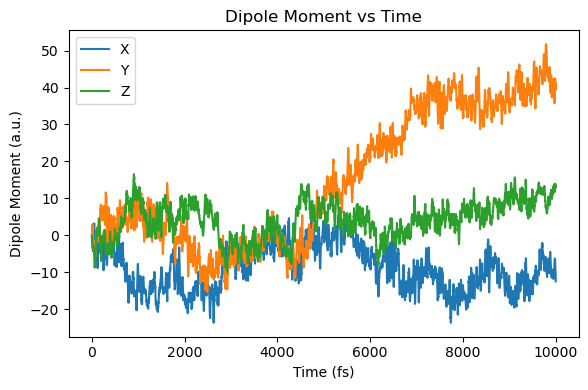
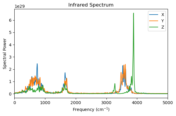
3. Plot IR spectrum of liquid water
[5]:
from maxwelllink.tools import ir_spectrum
import matplotlib.pyplot as plt

fs_to_au = 1 / 0.02418884254

mux = np.array([ad["mux_au"] for ad in molecule.additional_data_history])
muy = np.array([ad["muy_au"] for ad in molecule.additional_data_history])
muz = np.array([ad["muz_au"] for ad in molecule.additional_data_history])
t = np.array([ad["time_au"] for ad in molecule.additional_data_history]) / fs_to_au

plt.figure(figsize=(6, 4))
plt.plot(t, mux, label="X")
plt.plot(t, muy, label="Y")
plt.plot(t, muz, label="Z")
plt.xlabel("Time (fs)")
plt.ylabel("Dipole Moment (a.u.)")
plt.title("Dipole Moment vs Time")
plt.legend()
plt.tight_layout()
plt.show()

freq, sp_x = ir_spectrum(mux, 0.5*time_units_fs/resolution, field_description="square")
freq, sp_y = ir_spectrum(muy, 0.5*time_units_fs/resolution, field_description="square")
freq, sp_z = ir_spectrum(muz, 0.5*time_units_fs/resolution, field_description="square")

plt.figure(figsize=(6, 4))
plt.plot(freq, sp_x, label="X")
plt.plot(freq, sp_y, label="Y")
plt.plot(freq, sp_z, label="Z")
plt.xlim(0, 5000)
plt.xlabel("Frequency (cm$^{-1}$)")
plt.ylabel("Spectral Power")
plt.title("Infrared Spectrum")
plt.legend()
plt.tight_layout()

plt.show()
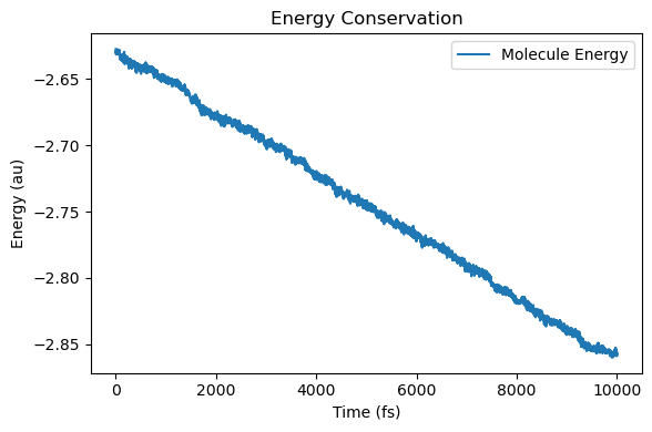
4. How to understand energy conservation?
We can also check energy conservation as below.
The energy of the molecular system is reduced because the molecular system is continuously emitting EM field.
If the absorbing boundary conditions for the EM field are turned off (as in # geometry 2 in the first code block), i.e., using the geometry below instead of a Bragg resonator with absorbing boundary conditions (PML):
length = 0.5 * rescaling
cell_size = mp.Vector3(length, 0, 0)
geometry = []
pml_layers = []
energy conservation for the molecular system should be greatly improved. The readers may have a try.
More importantly, when a larger water system is coupled to the cavity with a smaller rescaling factor, the IR emission of the molecular system will be greatly reduced, thus also improving energy conservation in the molecular system.
[6]:
# also plot energy conservation dynamics
energy_molecule = np.array([ad["energy_au"] for ad in molecule.additional_data_history])

plt.figure(figsize=(6, 4))
plt.plot(t, energy_molecule, label="Molecule Energy")
plt.xlabel("Time (fs)")
plt.ylabel("Energy (au)")
plt.title("Energy Conservation")
plt.legend()
plt.tight_layout()