Spontaneous emission of TLS: TCP socket
Here, we introduce the two-level system (TLS) spontaneous emission tutorial using maxwelllink.Molecule and a TCP socket.
1. Setting up the socket communication layer
Using the TCP socket requires to set the hostname and port number. In local machines, we can use the helper function get_available_host_port() from MaxwellLink to obtain these two pieces of information. Then, we initialize a SocketHub instance to provide the socket communication in MaxwellLink.
[1]:
import numpy as np
import maxwelllink as mxl
from maxwelllink import sockets as mxs

try:
    import meep as mp
except ImportError as exc:
    raise RuntimeError(
        "Meep is required for this tutorial."
        "Install via conda: conda install -c conda-forge pymeep=*=mpi_mpich_*"
    ) from exc

host, port = mxs.get_available_host_port()
hub = mxl.SocketHub(host=host, port=port, timeout=10.0, latency=1e-5)

print(f"SocketHub listening on {host}:{port}")
SocketHub listening on 127.0.0.1:49633
2. Bind Molecule and EM solver to the SocketHub
Then, we create a Molecule instance to define the information of this molecule in the EM simulation environment, including the center, size, sigma (width of the molecular polarization distribution), and dimensions.
We also need to setup the EM solver (MEEP) using mxl.MeepSimulation. This class is a wrapper of the meep.Simulation object with extended parameters for MaxwellLink.
[2]:
molecule = mxl.Molecule(
    hub=hub,
    center=mp.Vector3(0, 0, 0),
    size=mp.Vector3(1, 1, 1),
    sigma=0.1,
    dimensions=2,
)

sim = mxl.MeepSimulation(
    hub=hub,
    molecules=[molecule],
    cell_size=mp.Vector3(8, 8, 0),
    boundary_layers=[mp.PML(3.0)],
    resolution=10,
    # fix a units system
    time_units_fs=0.1,
)
[Init Molecule] Under socket mode, registered molecule with ID 0


 ######### MaxwellLink Units Helper #########
 MEEP uses its own units system, which is based on the speed of light in vacuum (c=1),
 the permittivity of free space (epsilon_0=1), and the permeability of free space (mu_0=1).
 To couple MEEP with molecular dynamics, we set [c] = [epsilon_0] = [mu_0] = [hbar] = 1.
 By further defining the time unit as 1.0000E-01 fs, we can fix the units system of MEEP (mu).

 Given the simulation resolution = 10,
 - FDTD dt = 5.0000E-02 mu (0.5/resolution) = 5.0000E-03 fs
 - FDTD dx = 1.0000E-01 mu (1.0/resolution) = 2.9979E+00 nm
 - Time [t]: 1 mu = 1.0000E-01 fs = 4.1341E+00 a.u.
 - Length [x]: 1 mu = 2.9979E+01 nm
 - EM wavelength of 1 mu, angular frequency omega = 2pi mu = 4.1375E+01 eV = 3.3371E+05 cm-1 = 1.5205E+00 a.u.
 - Note that sources and dielectrics defined in MEEP use rotational frequency (f=omega/2pi),
 - so probabably we need covert 1 eV photon energy to rotational frequency f = 2.4169E-02 mu
 - Electric field [E]: 1 mu = 6.6486E+07 V/m = 1.2930E-04 a.u.
 Hope this helps!
 ############################################
3. Python way to lunch mxl_driver on a separate terminal
Generally, using the Socket Interface requires to launch the EM simulation in one terminal and then start the molecular driver simulation in a separate terminal. To avoid openning a second terminal, below we introduce a python helper function launch_tls_driver(...), which will launch mxl_driver from Python (so we can stay within this notebook to finish this tutorial).
Here, we set the TLS starting at the initial excited-state population of 1e-4.
Immediately after launching this driver in the background, we run the simulation using sim.run(...). This function is a wrapper of the meep.Simulation.run(...) function, which can accept user-defined step functions.
[3]:
import shlex
import shutil
import subprocess
import time


def launch_tls_driver(host: str, port: int, sleep_time: float = 0.5):
    executable = shutil.which('mxl_driver')
    if executable is None:
        raise RuntimeError('mxl_driver executable not found in PATH.')
    cmd = (
        f"{executable} --model tls --address {host} --port {port}"
        f' --param "omega=0.242, mu12=187, orientation=2, pe_initial=1e-4"'
    )
    print('Launching TLS driver via subprocess...')
    print('If you prefer to run it manually, execute:')
    print('  ' + cmd)
    argv = shlex.split(cmd)
    proc = subprocess.Popen(argv)
    time.sleep(sleep_time)
    return proc

launch_tls_driver(host, port)

sim.run(until=400)
Launching TLS driver via subprocess...
If you prefer to run it manually, execute:
  /Users/taoli/miniforge3/envs/mxl/bin/mxl_driver --model tls --address 127.0.0.1 --port 49633 --param "omega=0.242, mu12=187, orientation=2, pe_initial=1e-4"
-----------
Initializing structure...
time for choose_chunkdivision = 0.000118017 s
Working in 2D dimensions.
Computational cell is 8 x 8 x 0 with resolution 10
time for set_epsilon = 0.00376892 s
-----------
[SocketHub] CONNECTED: mol 0 <- 127.0.0.1:49636
[initialization] Time step in atomic units: 0.20670686667500004
[initialization] Assigned a molecular ID: 0
init TLSModel with dt = 0.206707 a.u., molecule ID = 0
[initialization] Finished initialization for molecular ID: 0
Meep progress: 228.10000000000002/400.0 = 57.0% done in 4.0s, 3.0s to go
on time step 4565 (time=228.25), 0.00087624 s/step
run 0 finished at t = 400.0 (8000 timesteps)
Received STOP, exiting
[SocketHub] DISCONNECTED: mol 0 from 127.0.0.1:49636
4. Retrieve molecular simulation data
After the simulation, we can retrieve molecular simulation data from molecule.extra, a Python dictionary which stores the molecular information sent from the driver code at each step of the simulation.
[ ]:
# users can also use molecule.additional_data_history to access the time-resolved data recorded during the simulation,
# population = np.array([entry["Pe"] for entry in molecule.additional_data_history])
# time_au = np.array([entry["time_au"] for entry in molecule.additional_data_history])
# but here we demonstrate the use of molecule.extra which is more convenient for post-processing and plotting.

population = molecule.extra["Pe"]
time_au = molecule.extra["time_au"]

print(f"Collected {population.size} samples.")
Collected 8001 samples.
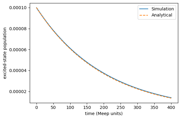
5. Compare with the Analytical Golden-Rule Decay
Finally, we can compare this numerical simulation with analytical golden-rule rate calculations, with the 2D spontaneus emission in vacuum as:
The corresponding TLS excited-state population decay dynamics obey:
When the EM field is described entirely classically, more than half a century ago, Jaynes and collaborators (https://ieeexplore.ieee.org/document/1443594) calculated the semiclassical spontaneous emission rate. More recently, we have also reproduced this semiclassical excited-state population decay (https://doi.org/10.1103/PhysRevA.97.032105):
When \(P_{\rm e}(0)\rightarrow 0\), the semiclassical decay dynamics exactly agree with the quantum correspondance \(P_{\rm e}^{\rm {QM}}(t)\).
As shown below, using \(P_{\rm e}(0)= 10^{-4}\), our semiclassical simulation exactly reproduces the quantum golden-rule decay.
[5]:
time_fs = time_au * 0.02418884254
time_meep = time_fs / 0.1
initial = population[0]
dipole_moment = 0.1 # meep units of mu12
frequency = 1.0 # meep units of omega

# analytical golden-rule decay rate
gamma = dipole_moment**2 * frequency**2 / 2.0

# simple exponential decay reference
reference = initial * np.exp(-time_meep * gamma)

# below is a more accurate reference which works under any initial population
#reference = np.exp(-time_meep * gamma) / (
#    np.exp(-time_meep * gamma) + (1.0 - initial) / initial
#)

std_rel = np.std(population - reference) / initial
max_rel = np.max(np.abs(population - reference)) / initial
print(f"std_dev={std_rel:.3e}, max_abs_diff={max_rel:.3e}")

import matplotlib.pyplot as plt

plt.figure(figsize=(6, 4))
plt.plot(time_meep, population, label="Simulation")
plt.plot(time_meep, reference, label="Analytical", linestyle="--")
plt.xlabel("time (Meep units)")
plt.ylabel("excited-state population")
plt.legend()
plt.tight_layout()
plt.show()
std_dev=2.012e-03, max_abs_diff=7.928e-03